Internet Problem Solving Contest

• Correct output – E1
• Correct output – E2
• C++ program to split input into biconnected components
• Python program solving processed data sets

The problem statement asks us to compute the expected cost of the minimum spanning tree of the given graph.

The graphs in the easy input were relatively small, and simpler to solve due to the fact that all the edge costs were chosen uniformly from [0,1].

The graphs in the hard input were larger. However, they shared one characteristics: they contained quite many articulation points, and had small biconnected components.

Note that when building the minimum spanning tree, we can split the graph into biconnected components, and compute the spanning tree separately for each of them. This is also obviously true for the expected cost in our setting.

Thus from now on we can concentrate on the main task: Given a relatively small graph, how to compute the expected cost of the minimum spanning tree?

Trees

For an edge with cost drawn randomly from [a,b], its expected cost is (a + b)∕2. If the input graph is a tree, we have to use all of its edges, and thus its expected cost is just the sum of the expected costs of all its edges.

Simulation

For really small graphs simulating the process a few times can be quite a good tool to get an idea how the expected cost behaves, and to use the approximated expected cost to check your program’s output later on.

However, the convergence rate of the simulation is pretty low, even after millions of attempts you will only get the first few significant digits of the expected cost, and this is nowhere near the accuracy needed to even guess the exact rational representation.

Notation

Let G be a graph. Its set of vertices will be denoted V (G), set of edges E(G).

Let Cost(G) be the cost of the minimum spanning tree of G (or ∞ if G is not connected), and κ(G) the number of connected components in G.

Given a graph G and a value t, let G[t] be the subgraph of G that contains all vertices of G, and exactly those edges whose cost is less than or equal to t.

Counting in a different way

Take a look at G[t]. What does it tell us about the minimum spanning tree? Imagine that you are building the spanning tree using Kruskal’s algorithm. After processing all edges with cost up to t inclusive, you will have a spanning forest for G[t]. What remains is to add some more edges to connect the components of G[t] into a single connected spanning tree.

Thus in the minimum spanning tree there are exactly κ(G[t]) - 1 edges more expensive than t. We can use this observation to write a different formula for the minimum spanning tree cost.

Let G be a connected graph where all edges have integer costs between 0 and C, inclusive. Then:

What we did here is simple: Consider an edge of the spanning tree, let its cost be c. The graphs G[0] to G[c- 1] do not contain this edge, and this causes these graphs to have one more connected component. Thus the total value of the sum is the sum of the costs of all edges in the spanning tree – i.e., the cost of the spanning tree.

We can easily generalize the formula to arbitrary real edge costs:

While this expression may be pretty clumsy for one fixed graph, it will be quite easy to adapt it to our situation.

Uniform edge costs

We will first show a solution for graphs with all edge costs from [0,1].

Let G be the input graph. Let H be a graph obtained from G by randomly generating the edge costs. For a fixed t [0,1] consider the graph H[t]. Let G′ be a graph obtained from G by erasing some (possibly zero) edges. What is the probability that G′ = H[t]?

This is simple: All the edges in E(G′) must have costs at most t, and all the others must have costs larger than t. Let M = |E(G)| = |E(H)| and M′ = |E(G′)|. Then the probability in question is prob(G′,t) = t^M′(1 - t)^M-M′.

Thus, given a value of t, we know the probability distribution for how H[t] looks like. This means that we can compute the expected number of components of H[t] simply by summing κ(G′)prob(G′,t) over all G′.

The result will be a polynomial with integer coefficients in t. We can then calculate the expected minimum spanning tree cost by using the formula for Cost(G) from the previous section.

Let the polynomial be q(t) = ∑ _i=0^Mq_itⁱ. Then:

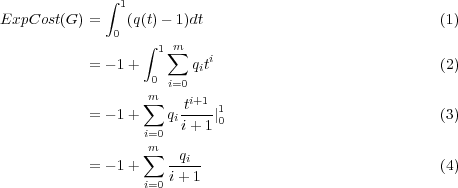
As all q_i were integers, this is a fraction, we just have to reduce and output it.

Different distributions of edge costs

As before, we want to evaluate the integral. However, in this case the probability distributions for H[t] given t are not polynomial any more. A simple way to overcome this obstacle is to split the interval of possible costs [0,C] into several smaller intervals. The splitting points will be the endpoints of probability distributions for each of the edges in G.

Evaluating the integral on one of the small intervals of costs, say [a,b], can be done in the same way as in the previous section: First, we have some edges that certainly are in H[t]. We add these, and merge the connected vertices. Second, we have some edges that are certainly too expensive to be in H[t]. We throw these away.

Last, we have edges that can have costs from (a,b). From the way how we chose the splitting points we know that for each such edge its interval of possible costs contains the entire interval [a,b]. As a consequence, on the interval [a,b] the function giving the probability that the edge cost of the given edge is lower than t is a rational polynomial in t. (This time, the coefficients of the resulting polynomial do not have to be integers any more, but they surely will be rational, and this is sufficient for us.)

This means that we can still use the same approach: Try all possibilities for the uncertain edges, compute the polynomial giving the expected number of connected components as a function of t, and then integrate this polynomial over the given interval of costs to get a part of the expected spanning tree cost.