
In the easy subproblem we are given a sorting routine that takes an n-element array and applies the following steps:
There is a special case that makes the solution work for n ≤ 2, but that’s it. On the first glance this seems pretty suspicious: does this ever work? But if we do a few experiments, we’ll discover that it does seem to work for all short arrays we throw at it.
Before we explain why it sorts and where it stops sorting correctly, we’ll describe a really simple approach that can solve this task without a full understanding of the implemented algorithm.
A trick that uses inductive reasoning
We will start by taking an educated guess that the worst possible input for an algorithm of this type will be an array sorted in reverse order. We could try this particular input for each n and see where it fails.
Well, that’s a good idea, but it’s not enough. The trouble here is that the algorithm is very inefficient and it would take ages to terminate for larger values of n.
Luckily for us, there is a very simple optimization. Suppose we already tried all input sizes smaller than the n we are now verifying. This means that whenever we call our function on an array of length smaller than n, the function will sort the array correctly. We can do the same thing much faster – simply by calling a standard O(nlogn)-time sort instead of making the recursive call. This change makes the whole routine run in O(nlogn), and therefore our search for the smallest counterexample will run in O(n2logn), which turns out to be fast enough.
Here’s a summary of this solution:
k1.{cc,py}.sort().A solution in which we understand what’s going on
OK, that was actually pretty cool, but some of us prefer to be sure that our solution is correct. What does the magic algorithm actually do?
The algorithm is a generalization of an esoteric sorting algorithm known as StoogeSort. In StoogeSort we always have a = b = c = ⌈2n/3⌉, and with this setting the algorithm is correct – but its time complexity is much worse than the quadratic time complexity of a dumb BubbleSort.
When exactly do these StoogeSort-like algorithms work correctly? Let’s draw a picture and use it to do some reasoning.
                             a
 first pass: |==============================|--------|

                                        b
second pass: |------------|==========================|

                           c                 n-c
 third pass: |=========================|-------------|
Imagine that we are doing a proof by induction (on n) that our algorithm correctly sorts any n-element array. The base case of the proof works: the algorithm has a special branch that makes it correct for n ≤ 2. Now let’s try proving the inductive step.
After the third pass we want to have a sorted array. According to the induction hypothesis, the third pass correctly sorts the first c elements. The output will be correct if and only if the last n − c elements were already the correct ones, and in their proper places. Let’s call these elements the large elements.
The second pass sorts the last b elements. This pass will put the large elements into their proper places if and only if all of them are among the last b elements of the array at the beginning of the second pass.
At the beginning some, possibly even all, large elements may be among the first a elements of the array. By sorting the first a elements we bring those large elements to the last few positions of the sorted part. All of them must belong to the part that will be sorted in the second pass. This means that the overlap between the first and the second pass must be at least as large as the total number of large elements.
(A more precise proof of the previous step would first show that a must be strictly greater than the number of large elements. Do you see why we should do that?)
And that’s it. The entire proof will work, as long as that last condition is satisfied. How does the condition look like in symbols? The length of the overlap between the first two passes is a + b − n. This must be at least as large as the number of large elements, which is n − c. In other words, we must have a + b + c ≥ 2n.
And that’s all there is to this problem. As long as we have a + b + c ≥ 2n, the routine sorts properly. And for the smallest n such that a + b + c < 2n, it is clearly enough to take a reversed array as a counterexample, because this array puts as many large elements as possible into the first a positions of the array.
Appendix
Did you wonder why is there a modulo operator in the definition of f3? The main purpose of this operator was to make life more difficult for solvers who would somehow try to binary search for the optimal counterexample. This tweak with %97 is there to make sure that the property we examine is not monotonous: after the correct counterexample there are still some larger input sizes that are sorted properly.
Oh, and the optimal counterexample modulo 97 gives remainder 95, not 96 as you might guess. Yes, we are evil :)
The program for this subproblem does two things. First, it generates an awful lot of swaps. This may seem scary, but the composition of all those swaps is simply some permutation of the input. Note that this permutation is the same for all arrays of the same length.
Then, the program generates a slightly smaller number of conditional swaps, i.e., instructions of the following form: “given x and y such that x < y, if A[x]>A[y], swap A[x] and A[y]”.
These instructions are called comparators, and they are the key ingredient in sorting networks: a simple class of oblivious parallel sorting algorithms.
Evaluating whether a sorting network sorts is a hard problem, but there is a nice algorithmic trick to it called the 0-1 principle: instead of trying all possible permutations of the input, it is enough to try all possible vectors of zeros and ones. This brings the time complexity of the test from the trivial $\hat{O}(n!)$ down to $\hat{O}(2^n)$.
Of course, this still means that in practice we can afford testing an algorithm for n = 20, or maybe n = 30 if we are willing to wait for a while. If we do this to our algorithm, we can verify that it correctly sorts up to n = 30. That’s nice to know, but not exactly what we wanted.
How can we proceed? Let’s try examining our sorting network. We can easily modify the program to print all the swaps it performs, and then we can draw those comparators. If you do that, you should see something that closely resembles a bitonic sorter. And that might give you an idea how to proceed.
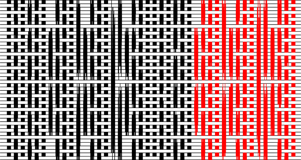
A plot of the swaps (black) and comparators (red) performed by our algorithm for n = 47.
In the comparator section of the plot there is only one single part (called “phase l, subphase l in our code) when the top half and bottom half get to mix. Let’s call this part”the big round“.
We can now divide the “wires” into the top half and the bottom half; for each half separately we can determine the possible outputs of the network before the big round. We will then get a very restricted set of possibilities for the input of the big round. And there, we have to check only two things:
Doing the above will allow us to find that the smallest n for which the network fails is n = 47.
For an alternate solution we may come up with an “educated guess” that a bad input for a network of mostly-random comparators could once again be a reversed array, or something similar to that. We can precompute (once) the permutation done by the first part of our algorithm, and then we can compute its inverse. That tells us the order in which to provide inputs in order to get a reversed array just before the swaps turn into comparators. And then it’s just a question of generating lots of inputs that resemble the reversed array, and feeding them into the implementation until you hit one that triggers the bug.